Modeling Transformer from scratch..
Every line of code, every reason behind it

Attention is a routing mechanism. By the time a token finishes its attention pass, its vector is no longer just its own representation — it’s a weighted mixture, pulled toward whatever it attended to. “Bank” has absorbed context from “river.” “It” has absorbed context from “trophy.”
But attention doesn’t reason about what it retrieved. It blends. It fetches. The actual processing of that blended signal happens in the next sublayer: the feed-forward network.
From ReLU to SwiGLU
The original Transformer used two linear layers with a ReLU between them. ReLU is simple: any negative value gets zeroed out, any positive value passes through unchanged. The problem is that hard zero. Neurons that consistently receive negative input stop contributing entirely — they’re dead, receiving no gradient, never updating. The kink at zero also makes the optimization landscape jagged.
Modern LLMs replaced ReLU with SiLU — the Sigmoid Linear Unit:
SiLU is smooth everywhere. For negative inputs it returns a small negative value rather than a hard zero, so neurons never fully die. It looks like a soft, slightly shifted ReLU and trains meaningfully better.
But there’s a further change: a gate.
After attention, a token's vector carries a blend of retrieved context. Not all of that context is equally relevant to every computation the feed-forward layer needs to perform. A gating mechanism lets the network learn to selectively amplify or suppress different parts of the signal — dynamically, based on the input itself. One linear branch acts as a gate, controlling how much of a second branch passes through. The gate learns what to let through. The value branch learns what to say.
Combining SiLU with this gating structure gives SwiGLU — the activation used in LLaMA 3, Qwen, and most modern LLMs:
Three weight matrices instead of two. W1 produces the gate. W3 produces the values. Their elementwise product is what W2 projects back to model dimension. Noam Shazeer, who proposed it, tested it against every alternative and found it consistently won. His explanation:
We offer no explanation as to why these architectures seem to work; we attribute their success, as all else, to divine benevolence.
The clearest insight comes from Geva et al. (2021), who showed that feed-forward layers behave like soft key-value memory stores — the first linear projection pattern-matches the input against learned keys, and the second retrieves associated values. Through that lens, the SwiGLU gate is a relevance filter on top of that retrieval: it amplifies keys that match the current input and suppresses those that don't, making the lookup sharper and more selective. The multiplicative interaction between the gate and value branches also gives the layer strictly more expressive power than a purely additive design, letting it represent functions that would otherwise require additional depth. It's not a complete explanation, but it's a principled one: the gate makes the FFN a better memory retrieval mechanism, not just a wider one.
One dimension detail worth knowing: the original two-matrix FFN used an inner dimension of 4 × dmodel. Adding a third matrix would increase parameter count by 50%. The fix is to shrink the inner dimension to 8/3 × dmodel — keeping total FFN parameters roughly equivalent. In practice you round to the nearest multiple of 64, since matrix multiplications run fastest when dimensions align to GPU memory boundaries.
import math
import torch
import torch.nn as nn
from torch import Tensor


class Linear(nn.Module):
    """
    Linear transformation y = Wx, with no bias term.

    Modern LLMs drop bias terms entirely — RMSNorm (which we'll build
    next) already handles scale, making bias redundant. Fewer parameters
    also means a simpler optimization landscape with no perplexity cost.

    Weight W is stored as (out_features, in_features) to match the
    mathematical convention y = Wx. The forward pass uses einsum to
    handle arbitrary leading batch dimensions cleanly.

    Args:
        in_features:  Dimensionality of input vectors.
        out_features: Dimensionality of output vectors.
        device:       Device to allocate the weight on.
        dtype:        Data type of the weight.
    """

    def __init__(
        self,
        in_features: int,
        out_features: int,
        device: torch.device | None = None,
        dtype: torch.dtype | None = None,
    ) -> None:
        super().__init__()
        self.weight = nn.Parameter(
            torch.empty(out_features, in_features, device=device, dtype=dtype)
        )
        # Glorot-style init: variance = 2/(in+out), truncated at ±3σ.
        # Keeps activation scale stable as signal passes through layers.
        sigma = math.sqrt(2.0 / (in_features + out_features))
        nn.init.trunc_normal_(
            self.weight, mean=0.0, std=sigma, a=-3 * sigma, b=3 * sigma
        )

    def forward(self, x: Tensor) -> Tensor:
        """
        Apply linear transformation to input.

        Args:
            x: Tensor of shape (..., in_features).

        Returns:
            Tensor of shape (..., out_features).
        """
        # Contracts over d_in, preserves all leading dims, produces d_out.
        return torch.einsum("...i,oi->...o", x, self.weight)


class SwiGLUFFN(nn.Module):
    """
    Position-wise Feed-Forward Network using SwiGLU activation.

    Implements: FFN(x) = W2 * (SiLU(W1 * x) ⊗ W3 * x)

    Applied identically and independently at every sequence position —
    no cross-token communication happens here. Attention is the
    conversation; this is each token thinking about what it just heard.

    Hidden dimension d_ff ≈ (8/3) * d_model rounded to the nearest
    multiple of 64. The (8/3) factor compensates for the extra W3
    matrix, keeping total parameter count equivalent to the original
    4 * d_model two-matrix design.

    Args:
        d_model: Input and output dimensionality.
        d_ff:    Inner dimensionality. If None, computed automatically.
        device:  Device for parameters.
        dtype:   Data type for parameters.
    """

    def __init__(
        self,
        d_model: int,
        d_ff: int | None = None,
        device: torch.device | None = None,
        dtype: torch.dtype | None = None,
    ) -> None:
        super().__init__()

        if d_ff is None:
            # Round (8/3)*d_model up to the nearest multiple of 64.
            d_ff = math.ceil(int(8 / 3 * d_model) / 64) * 64

        # Gate branch: its output controls what information passes through.
        self.W1 = Linear(d_model, d_ff, device=device, dtype=dtype)

        # Output projection: maps the gated result back to d_model.
        self.W2 = Linear(d_ff, d_model, device=device, dtype=dtype)

        # Value branch: the content being selectively passed through.
        self.W3 = Linear(d_model, d_ff, device=device, dtype=dtype)

    def forward(self, x: Tensor) -> Tensor:
        """
        Apply SwiGLU feed-forward transformation.

        Args:
            x: Input of shape (batch_size, seq_len, d_model).

        Returns:
            Output of shape (batch_size, seq_len, d_model).
        """
        # Compute W1(x) once and cache — used for both the gate value
        # and the SiLU nonlinearity. SiLU = x * σ(x): smooth, never
        # produces a hard zero, so no neurons permanently die.
        gate_input = self.W1(x)
        gate = gate_input * torch.sigmoid(gate_input)

        # Values: the content the gate decides how much of to pass through.
        values = self.W3(x)

        # Elementwise product: each dimension independently gated.
        # The network learns which channels to amplify or suppress
        # as a function of the input — dynamic feature selection.
        return self.W2(gate * values)
RMSNorm — and Why Where You Put It Matters
As activations pass through many layers, their scale drifts. Vectors that started with reasonable magnitudes can explode or shrink, depending on what the weight matrices do to them. When that happens, gradients misbehave — either vanishing entirely in early layers or blowing up into numerical instability.
Normalization fixes this by rescaling the activation vector at each position back to a controlled magnitude before passing it to the next operation. The original Transformer used LayerNorm, which normalizes by subtracting the mean and dividing by the standard deviation. Modern LLMs use RMSNorm — Root Mean Square Normalization — which drops the mean subtraction entirely:
Why drop the mean subtraction? It turns out most of the stabilizing effect of LayerNorm comes from the variance normalization, not the centering. The mean subtraction adds compute and parameters without meaningfully improving results. LLaMA, GPT-NeoX, and most post-2022 models use RMSNorm for this reason.
The g term is a learned per-dimension gain, initialized to all ones so RMSNorm starts as an identity rescaling and the model learns from there. The ε is a small constant — typically 1e-5— that prevents division by zero when activations are near zero.
Pre-norm vs post-norm — the decision that changed training
Where you place normalization matters as much as which normalization you use.
The original Transformer normalized after each sublayer — apply attention or FFN, add the residual, then normalize:
output = LayerNorm(x + SubLayer(x)) ← post-normModern models normalize before — normalize first, apply the sublayer, then add the original input back:
output = x + SubLayer(RMSNorm(x)) ← pre-normThis seemingly small change has a large effect on training stability. In post-norm, the normalization sits inside the residual path. During early training when norms are large, this gates the gradient flowing through the shortcut connection — the very connection that is supposed to guarantee gradient flow to early layers gets partially blocked. Post-norm models famously require careful learning rate warmup schedules to avoid instability at the start of training.
In pre-norm, there is a clean residual stream from input to output with no normalization inside it. Gradients flow all the way back to early layers through the residual connections without passing through any gating. The shortcut does what it was designed to do. Pre-norm models often train stably without warmup, and this architecture — used in GPT-3, LLaMA, PaLM, and essentially every large model since 2020 — is now the standard.
The cost is minimal: one extra RMSNorm after the final Transformer block, since pre-norm only normalizes each sublayer’s input, not its output.
class RMSNorm(nn.Module):
    """
    Root Mean Square Layer Normalization (Zhang & Sennrich, 2019).

    Normalizes by RMS rather than standard deviation — no mean subtraction.
    This is cheaper than LayerNorm and empirically equivalent for LLMs.

    The learnable gain g (initialized to ones) lets the model rescale
    each dimension independently after normalization. It starts as an
    identity so the network learns deviations from there.

    We upcast to float32 before squaring to prevent overflow with fp16
    or bf16 inputs, then restore the original dtype before returning.

    Args:
        d_model: Dimensionality of the input vectors.
        eps:     Small constant for numerical stability (default: 1e-5).
        device:  Device to allocate the gain parameter on.
        dtype:   Data type of the gain parameter.
    """

    def __init__(
        self,
        d_model: int,
        eps: float = 1e-5,
        device: torch.device | None = None,
        dtype: torch.dtype | None = None,
    ) -> None:
        super().__init__()
        self.eps = eps
        # Gain initialized to ones: starts as identity rescaling.
        # Shape (d_model,) broadcasts over batch and sequence dimensions.
        self.weight = nn.Parameter(
            torch.ones(d_model, device=device, dtype=dtype)
        )

    def forward(self, x: Tensor) -> Tensor:
        """
        Apply RMSNorm to the last dimension of x.

        Args:
            x: Input tensor of shape (..., d_model).

        Returns:
            Normalized tensor of the same shape, in the original dtype.
        """
        # Store original dtype — we'll restore it before returning.
        in_dtype = x.dtype

        # Upcast to float32 before squaring. Large fp16/bf16 values
        # can overflow when squared, producing inf and breaking training.
        x = x.to(torch.float32)

        # Compute RMS across the last dimension (d_model).
        # keepdim=True preserves the dimension for broadcasting.
        rms = torch.sqrt(x.pow(2).mean(dim=-1, keepdim=True) + self.eps)

        # Normalize, then apply the learned per-dimension gain.
        result = (x / rms) * self.weight.to(torch.float32)

        # Restore original dtype before returning.
        return result.to(in_dtype)
The Residual Connection
Before residual connections, training networks deeper than roughly twenty layers was nearly impossible in practice. The reason is the same one that makes RNNs struggle with long sequences: the vanishing gradient problem. During backpropagation, gradients are computed by repeatedly applying the chain rule — multiplying Jacobians together, one per layer. If those Jacobians have values consistently less than one, the product shrinks exponentially with depth. By the time the gradient reaches early layers, there is almost nothing left. The early layers stop learning. The network effectively becomes shallow regardless of how many layers you stacked.
The fix, introduced in ResNets in 2015, is almost embarrassingly simple. Instead of each layer computing a full new representation from scratch, it computes a correction to the existing one:
output = x + SubLayer(x)That single + changes everything. Gradients now have two paths back through each block — through the sublayer, and directly through the addition. The direct path carries the gradient unchanged, no matter how many layers deep you are. Early layers always receive a usable gradient signal. You can stack a hundred layers and training still works.
There is a deeper way to think about this. Without residuals, each layer transforms the representation — the input goes in, something different comes out. With residuals, each layer adds to a shared stream. Every block reads from the same stream and writes a small delta back. The representation is not replaced at each layer; it is incrementally refined. Early layers establish coarse structure. Later layers make fine corrections. The stream accumulates meaning as it flows through the network.
This framing — the residual stream — is also the foundation of mechanistic interpretability research. When researchers talk about attention heads that “read from” and “write to” specific dimensions, or about circuits that activate in certain layers, they are talking about operations on this stream. The residual connection is what makes the transformer legible at all.
Attention step by step
In the last post we walked through attention step by step — the query, key, value projections, the scaled dot product, the softmax, the causal mask. Here we build it.
Softmax first, because attention depends on it — and because the naive implementation breaks with large inputs:
def softmax(x: Tensor, dim: int) -> Tensor:
    """
    Numerically stable softmax along a specified dimension.

    The naive implementation — exp(x) / sum(exp(x)) — overflows when
    any value in x is large, producing inf and then nan. The fix: softmax
    is invariant to subtracting a constant from all inputs (the constant
    cancels in numerator and denominator), so we subtract the max first,
    making the largest pre-exp value exactly zero and all others negative.

    Args:
        x:   Input tensor of arbitrary shape.
        dim: Dimension along which to compute softmax.

    Returns:
        Tensor of same shape as x, summing to 1 along dim.
    """
    # Subtract max for numerical stability — no change to the output,
    # but prevents overflow when exponentiating large values.
    x_shifted = x - x.max(dim=dim, keepdim=True).values
    exp_x = torch.exp(x_shifted)
    return exp_x / exp_x.sum(dim=dim, keepdim=True)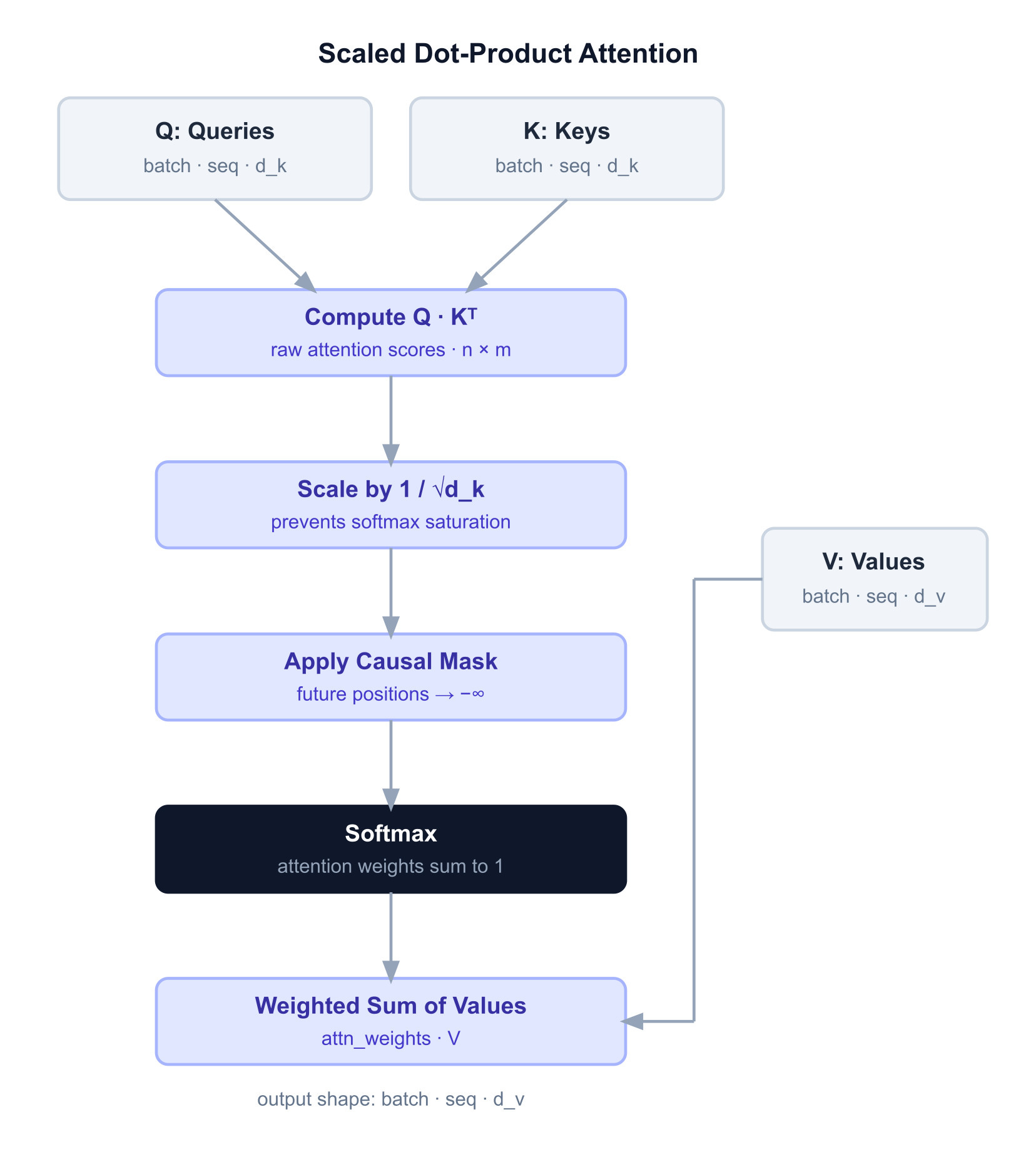
def scaled_dot_product_attention(
    query: Tensor,
    key: Tensor,
    value: Tensor,
    mask: Tensor | None = None,
) -> Tensor:
    """
    Scaled dot-product attention: softmax(QK^T / sqrt(d_k)) * V

    The scaling by sqrt(d_k) prevents softmax saturation. Without it,
    dot products grow with dimension size — large scores push softmax
    toward one-hot distributions with near-zero gradients, stalling
    training. Dividing by sqrt(d_k) keeps variance at 1 regardless
    of dimension size.

    The optional mask enforces causal attention in decoder models:
    position i is only allowed to attend to positions j <= i.
    Masked positions receive -inf before softmax, which becomes
    exactly zero weight after exponentiation.

    Args:
        query: Tensor of shape (..., seq_len, d_k).
        key:   Tensor of shape (..., seq_len, d_k).
        value: Tensor of shape (..., seq_len, d_v).
        mask:  Optional boolean tensor of shape (seq_len, seq_len).
               True = attend, False = block (set to -inf).

    Returns:
        Tensor of shape (..., seq_len, d_v).
    """
    d_k = query.shape[-1]

    # Compute raw attention scores: how much does each query
    # want to attend to each key? Result shape: (..., seq_len, seq_len)
    scores = scores = torch.einsum("...nd,...md->...nm", query, key)

    # Scale to prevent softmax saturation as d_k grows.
    scores = scores / math.sqrt(d_k)

    # Apply causal mask: blocked positions become -inf so softmax
    # maps them to exactly zero weight.
    if mask is not None:
        scores = scores.masked_fill(~mask, float("-inf"))

    # Softmax over the key dimension — converts scores to weights
    # that sum to 1 across all positions attended to.
    attn_weights = softmax(scores, dim=-1)

    # Weighted sum of value vectors: each output position gets
    # a blend of values, weighted by attention.
    return torch.einsum("...nm,...mv->...nv", attn_weights, value)
One subtlety before we implement the Multi-Head Attention: attention has no inherent sense of position. Without positional information, shuffling the input tokens in any order would produce the same output — just shuffled. Position has to be injected. We use RoPE — Rotary Positional Embeddings. We covered how RoPE works in my second post on embeddings — rotations rather than additions, relative rather than absolute positions. Here's the implementation:
class RotaryPositionalEmbedding(nn.Module):
    """
    Rotary Positional Embeddings (RoPE), Su et al. 2021.

    Encodes position by rotating query and key vectors by position-
    dependent angles. The dot product q_i · k_j then depends only on
    the relative offset (i - j), not absolute positions — making
    attention naturally position-relative.

    No learned parameters: the rotation angles are fixed by the
    architecture. Precomputed cos/sin tables are stored as buffers
    (they move with the model but are not updated by the optimizer).

    Args:
        theta:       Base frequency (Θ). Typically 10000.0.
        d_k:         Dimension of query/key vectors. Must be even.
        max_seq_len: Maximum sequence length for precomputation.
        device:      Device to store the buffers on.
    """

    def __init__(
        self,
        theta: float,
        d_k: int,
        max_seq_len: int,
        device: torch.device | None = None,
    ) -> None:
        super().__init__()
        assert d_k % 2 == 0, "d_k must be even for RoPE"

        # Frequencies: theta^(-(2k)/d_k) for k = 0 ... d_k/2 - 1.
        # Low-index pairs rotate fast (high frequency).
        # High-index pairs rotate slow (low frequency).
        k = torch.arange(0, d_k // 2, dtype=torch.float32, device=device)
        inv_freq = 1.0 / (theta ** (2 * k / d_k))  # (d_k/2,)

        # Precompute angles for every (position, pair) combination.
        positions = torch.arange(max_seq_len, dtype=torch.float32, device=device)
        angles = torch.outer(positions, inv_freq)   # (max_seq_len, d_k/2)

        # Duplicate so each angle covers both dimensions in its pair.
        angles = torch.cat([angles, angles], dim=-1)  # (max_seq_len, d_k)

        # Register as non-learned buffers — travel with the model,
        # not updated by the optimizer.
        self.register_buffer("cos_cache", angles.cos(), persistent=False)
        self.register_buffer("sin_cache", angles.sin(), persistent=False)

    def _rotate_half(self, x: Tensor) -> Tensor:
        """
        Maps (x1, x2, x3, x4, ...) → (-x2, x1, -x4, x3, ...).

        Combined with cos/sin multiplication, this implements a 2D
        rotation on each consecutive pair of dimensions — without
        constructing the full rotation matrix.
        """
        half = x.shape[-1] // 2
        return torch.cat([-x[..., half:], x[..., :half]], dim=-1)

    def forward(self, x: Tensor, token_positions: Tensor) -> Tensor:
        """
        Apply RoPE rotation to a query or key tensor.

        Rotation formula: x' = x * cos(θ) + rotate_half(x) * sin(θ)
        This is equivalent to a 2D rotation on each dimension pair,
        derived from expanding the rotation matrix multiplication.

        Args:
            x:               Tensor of shape (..., seq_len, d_k).
            token_positions: Integer tensor of shape (..., seq_len).

        Returns:
            Rotated tensor of same shape as x.
        """
        cos = self.cos_cache[token_positions]  # (..., seq_len, d_k)
        sin = self.sin_cache[token_positions]  # (..., seq_len, d_k)
        return x * cos + self._rotate_half(x) * sin
Multi-head attention sounds complex. The implementation collapses to three matrix multiplies and a reshape.
Instead of running a separate projection for each head, we project the full d_model dimension in one shot — then slice it into h equal chunks, one per head. Each head gets its own slice of Q, K, and V to work with, runs attention independently, and produces its own output. RoPE rotates the queries and keys so attention is sensitive to how far apart two tokens are. A lower-triangular mask makes sure no token can peek at tokens ahead of it. Finally, we stitch all the head outputs back together and run one last projection to mix what each head found.
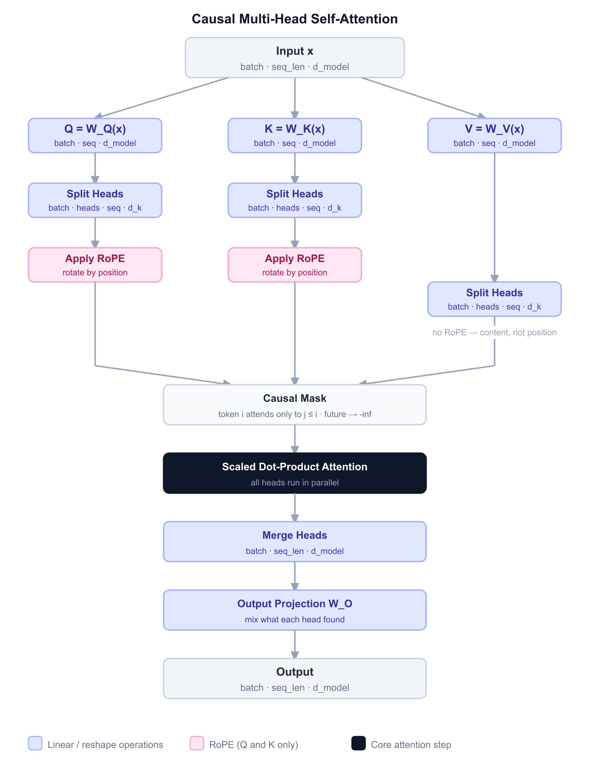
Why no RoPE on V? RoPE’s job is to help tokens find each other. When a query at position 5 looks for a key at position 2, the rotation encodes that they are 3 apart — shaping the attention score. Position matters for the search.
Once a token has been found, what it says should not depend on where it sits. The content a token communicates when attended to is the same regardless of position. Q and K do the finding. V does the talking.
class CausalMultiHeadSelfAttention(nn.Module):
    """
    Multi-Head Self-Attention with causal masking and RoPE.

    Every token attends to every other token — but only to tokens
    that came before it, never ahead. Multiple heads run in parallel,
    each learning to attend to different kinds of relationships.

    Args:
        d_model:     Size of each token's vector.
        num_heads:   How many attention heads to run in parallel.
        max_seq_len: Longest sequence we'll ever see (needed for RoPE).
        theta:       RoPE frequency parameter. Default 10000.0.
        device:      Where to store the weights.
        dtype:       Weight data type.
    """

    def __init__(
        self,
        d_model: int,
        num_heads: int,
        max_seq_len: int,
        theta: float = 10000.0,
        device: torch.device | None = None,
        dtype: torch.dtype | None = None,
    ) -> None:
        super().__init__()
        assert d_model % num_heads == 0, "d_model must be divisible by num_heads"

        self.d_model = d_model
        self.num_heads = num_heads
        self.d_k = d_model // num_heads  # each head works in this smaller space

        # Three projections: what each token is looking for (Q),
        # what it offers to others (K), and what it says when found (V).
        self.W_Q = Linear(d_model, d_model, device=device, dtype=dtype)
        self.W_K = Linear(d_model, d_model, device=device, dtype=dtype)
        self.W_V = Linear(d_model, d_model, device=device, dtype=dtype)

        # After all heads are done, combine their outputs back into one vector.
        self.W_O = Linear(d_model, d_model, device=device, dtype=dtype)

        # RoPE rotates Q and K based on position so attention
        # is sensitive to how far apart two tokens are.
        self.rope = RotaryPositionalEmbedding(
            theta=theta,
            d_k=self.d_k,
            max_seq_len=max_seq_len,
            device=device,
        )

    def forward(self, x: Tensor) -> Tensor:
        batch_size, seq_len, _ = x.shape

        # Step 1 — project input into Q, K, V spaces
        Q = self.W_Q(x)   # what each token is looking for
        K = self.W_K(x)   # what each token offers to match against
        V = self.W_V(x)   # what each token communicates if attended to

        # Step 2 — split into heads
        # each head gets its own slice of the embedding dimension
        # shape goes from (batch, seq, d_model) → (batch, heads, seq, d_k)
        def split_heads(t):
            t = t.view(batch_size, seq_len, self.num_heads, self.d_k)
            return t.transpose(1, 2)

        Q = split_heads(Q)
        K = split_heads(K)
        V = split_heads(V)

        # Step 3 — rotate Q and K by position using RoPE
        # this makes attention aware of how far apart tokens are
        # V is not rotated — position matters for finding, not for content
        positions = torch.arange(seq_len, device=x.device)
        Q = self.rope(Q, positions)
        K = self.rope(K, positions)

        # Step 4 — build the causal mask
        # token i can only attend to tokens at positions j <= i
        # anything above the diagonal gets blocked
        causal_mask = torch.tril(
            torch.ones(seq_len, seq_len, dtype=torch.bool, device=x.device)
        )

        # Step 5 — run attention for all heads at once
        # the head dimension just batches naturally here
        attn_out = scaled_dot_product_attention(Q, K, V, mask=causal_mask)

        # Step 6 — merge all heads back into one vector per token
        # (batch, heads, seq, d_k) → (batch, seq, d_model)
        attn_out = attn_out.transpose(1, 2).contiguous()
        attn_out = attn_out.view(batch_size, seq_len, self.d_model)

        # Step 7 — final projection to mix what each head found
        return self.W_O(attn_out)
Putting it all together - The Transformer Block
A Transformer block applies two sublayers in sequence. Each follows the same pattern: normalize the input, run the operation, add the result back to what came in. That addition is the residual connection — the shortcut that keeps gradients flowing through the whole stack.
The first sublayer lets tokens talk to each other. The second lets each token think about what it just heard. Together they form one complete block, repeated identically across all layers.
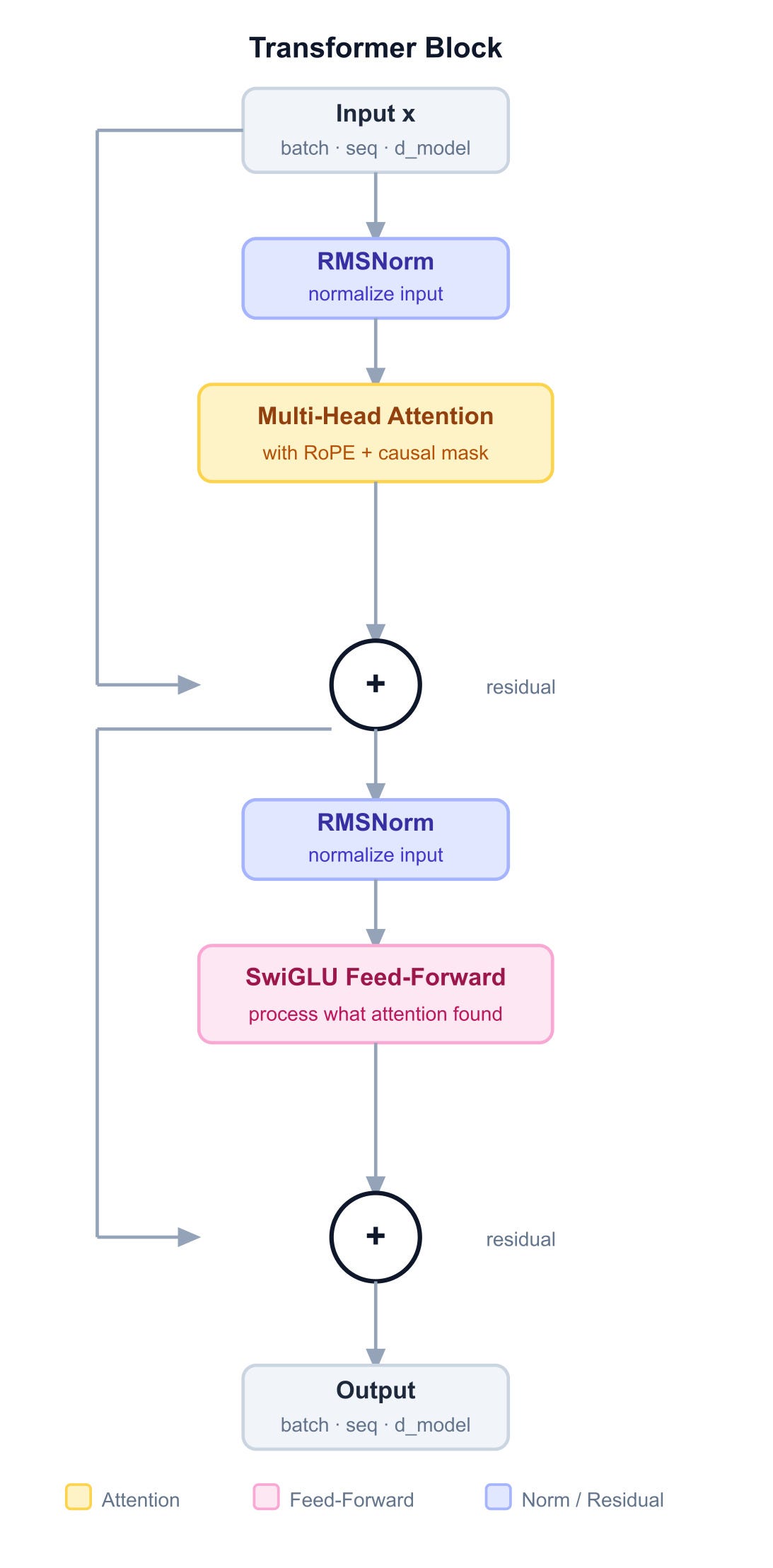
class TransformerBlock(nn.Module):
    """
    One Transformer block: attention followed by feed-forward,
    each wrapped in a pre-norm residual sublayer.

    The pattern for each sublayer is:
        x = x + SubLayer(RMSNorm(x))

    Normalizing before the operation (pre-norm) keeps the residual
    stream clean — gradients flow back through the addition without
    passing through any normalization, making deep stacks trainable.

    Args:
        d_model:     Size of each token's vector.
        num_heads:   Number of attention heads.
        d_ff:        Inner dimension of the feed-forward network.
        max_seq_len: Longest sequence we'll ever process.
        theta:       RoPE base frequency. Default 10000.0.
        device:      Where to store the weights.
        dtype:       Weight data type.
    """

    def __init__(
        self,
        d_model: int,
        num_heads: int,
        d_ff: int,
        max_seq_len: int,
        theta: float = 10000.0,
        device: torch.device | None = None,
        dtype: torch.dtype | None = None,
    ) -> None:
        super().__init__()

        # Normalize before attention
        self.norm1 = RMSNorm(d_model, device=device, dtype=dtype)

        # Tokens talk to each other
        self.attn = CausalMultiHeadSelfAttention(
            d_model=d_model,
            num_heads=num_heads,
            max_seq_len=max_seq_len,
            theta=theta,
            device=device,
            dtype=dtype,
        )

        # Normalize before feed-forward
        self.norm2 = RMSNorm(d_model, device=device, dtype=dtype)

        # Each token thinks about what it just heard
        self.ffn = SwiGLUFFN(d_model=d_model, d_ff=d_ff, device=device, dtype=dtype)

    def forward(self, x: Tensor) -> Tensor:
        """
        Args:
            x: (batch_size, seq_len, d_model)

        Returns:
            (batch_size, seq_len, d_model)
        """
        # Sublayer 1: normalize, attend, add back
        x = x + self.attn(self.norm1(x))

        # Sublayer 2: normalize, process, add back
        x = x + self.ffn(self.norm2(x))

        return x
The Full Transformer Language Model
Every piece is built. Now we stack them.
The language model is three stages: embed the token IDs into vectors, pass them through N identical Transformer blocks, then project to logits over the vocabulary. One detail worth noting — because we use pre-norm, the final block’s output has never been normalized. A last RMSNorm fixes that before the projection.
class TransformerLM(nn.Module):
    """
    Autoregressive Transformer Language Model.

    Takes a sequence of token IDs and predicts the next token
    at every position. At training time all positions are used.
    At inference time only the last position's logits matter.

    Architecture:
        token IDs → Embedding → [TransformerBlock × num_layers]
                  → RMSNorm → Linear → logits

    The final RMSNorm is needed because pre-norm only normalizes
    each sublayer's input, not its output. Without it, the last
    block's output lands directly on the projection — unnormalized.

    Args:
        vocab_size:     Number of tokens in the vocabulary.
        context_length: Maximum sequence length.
        d_model:        Size of each token's vector.
        num_layers:     Number of stacked Transformer blocks.
        num_heads:      Attention heads per block.
        d_ff:           FFN inner dimension. Defaults to (8/3)*d_model.
        theta:          RoPE base frequency. Default 10000.0.
        device:         Where to store the weights.
        dtype:          Weight data type.
    """

    def __init__(
        self,
        vocab_size: int,
        context_length: int,
        d_model: int,
        num_layers: int,
        num_heads: int,
        d_ff: int | None = None,
        theta: float = 10000.0,
        device: torch.device | None = None,
        dtype: torch.dtype | None = None,
    ) -> None:
        super().__init__()

        if d_ff is None:
            d_ff = math.ceil(int(8 / 3 * d_model) / 64) * 64

        # Stage 1: convert token IDs to vectors
        self.token_embedding = Embedding(
            num_embeddings=vocab_size,
            embedding_dim=d_model,
            device=device,
            dtype=dtype,
        )

        # Stage 2: stack of identical Transformer blocks
        # ModuleList registers each block so their parameters
        # appear in model.parameters() and move with .to(device)
        self.blocks = nn.ModuleList([
            TransformerBlock(
                d_model=d_model,
                num_heads=num_heads,
                d_ff=d_ff,
                max_seq_len=context_length,
                theta=theta,
                device=device,
                dtype=dtype,
            )
            for _ in range(num_layers)
        ])

        # Normalize the final block's output before projection
        self.final_norm = RMSNorm(d_model, device=device, dtype=dtype)

        # Stage 3: project from d_model to vocabulary size
        self.lm_head = Linear(d_model, vocab_size, device=device, dtype=dtype)

    def forward(self, token_ids: Tensor) -> Tensor:
        """
        Args:
            token_ids: (batch_size, seq_len) integer token IDs

        Returns:
            logits: (batch_size, seq_len, vocab_size)
            logits[b, i, :] is the predicted distribution over
            the next token after position i in batch element b.
        """
        # Embed token IDs into vectors
        x = self.token_embedding(token_ids)

        # Pass through each Transformer block
        for block in self.blocks:
            x = block(x)

        # Normalize before projecting
        x = self.final_norm(x)

        # Project to vocabulary logits
        return self.lm_head(x)
What We’ve Actually Built
We started this post with a stack of disconnected ideas — a normalization trick, a gating mechanism, a rotation matrix — and ended with a language model. The same architectural skeleton that GPT, LLaMA, and Mistral are built on.
Every piece had a reason. RMSNorm before, not after, because the residual stream needs to stay free. SwiGLU because a gate that learns whether to pass information is more expressive than one that just clips negatives. RoPE on queries and keys but not values, because position is about where to look, not what to say. Residual connections because without them, gradients dissolve before they reach layer one.
None of these are accidents. Modern LLM architecture is decades of empirical pain compressed into elegant defaults.
What we cannot do yet: train it. You have the forward pass — the machine that turns tokens into logits. The backward pass, the optimizer, the data pipeline — that is a different story.
That story is next.
The complete code from this post is available as a Google Colab notebook — every component in one place, ready to run.